---
title: "Stage 2 · Fair Partner Comparison"
subtitle: "Case-mix adjustment · O/E ratios · Partial pooling · Funnel plot"
---
```{r setup}
#| include: false
library(tidyverse)
library(lme4)
library(mirai)
library(plotly)
library(gt)
library(patchwork)
library(ggeffects)
library(performance)
library(parameters)
library(effectsize)
library(sjPlot)
library(gtsummary)
library(gtExtras)
source("../R/utils_viz.R")
source("../R/utils_kpi.R")
source("../R/utils_models.R")
claims <- readRDS("../data/claims.rds")
partners <- readRDS("../data/partners.rds")
claims_steered <- claims |> filter(steering_flag == 1L, !is.na(partner_id))
```
## The Selection Bias Problem
Raw cost comparisons between partners are meaningless without adjustment: partners handling
complex, high-severity claims will appear expensive — not because they are inefficient,
but because of case mix.
```{r naive-comparison}
#| fig-height: 4
naive_stats <- claims_steered |>
  group_by(partner_id) |>
  summarise(
    avg_cost      = mean(repair_cost),
    n_claims      = n(),
    avg_severity  = mean(severity_score),
    .groups       = "drop"
  ) |>
  left_join(partners |> select(partner_id, name, type, region), by = "partner_id")

p_naive <- ggplot(naive_stats, aes(x = avg_severity, y = avg_cost,
                                    size = n_claims, colour = type)) +
  geom_point(alpha = 0.65, stroke = 0) +
  scale_colour_manual(values = c(
    Werkstatt   = "#003781", Glaspartner = "#0066CC",
    Gutachter   = "#00A9CE", Abschlepp   = "#66B5E8", Mietwagen   = "#FF6600"
  ), name = "Type") +
  scale_size_continuous(range = c(2, 9), guide = "none") +
  scale_y_continuous(labels = scales::label_number(prefix = "CHF ", big.mark = ",")) +
  labs(title    = "Naive Cost vs. Case Severity",
       subtitle = "Partners handling tougher cases appear more expensive — selection bias",
       x = "Avg. Severity Score", y = "Avg. Repair Cost") +
  theme_allianz()

ggplotly(p_naive, tooltip = c("x", "y"))
```
## Case-Mix Adjustment: GLM per Claim Type
Fit a GLM (gamma family, log link) for each claim type using `mirai` parallel workers.
The model regresses cost on vehicle class, vehicle age, severity score, and region.
```{r glm-parallel}
#| cache: false
daemons(4)

# Fit one GLM per claim type in parallel
claim_types_list <- levels(claims_steered$claim_type)

glm_results <- mirai_map(
  claim_types_list,
  function(ct, data) {
    df <- data[data$claim_type == ct, ]
    m  <- glm(
      repair_cost ~ vehicle_class + vehicle_age + severity_score + region,
      data   = df,
      family = Gamma(link = "log")
    )
    list(type = ct, model = m, n = nrow(df))
  },
  .args = list(data = claims_steered)
)

models_by_type <- setNames(
  lapply(glm_results[], `[[`, "model"),
  claim_types_list
)

daemons(0)
cat("GLMs fitted:", length(models_by_type), "models\n")
```
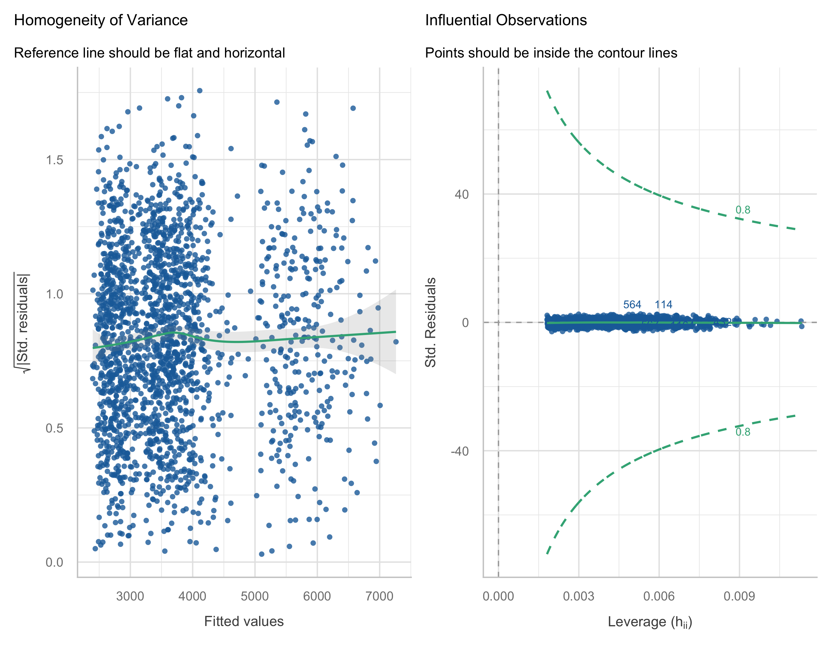
### Model Diagnostics
```{r model-diagnostics}
#| fig-height: 7
# Show diagnostics for body damage (largest segment)
m_body <- models_by_type[["body"]]
check_model(m_body, check = c("qq", "outliers", "homogeneity", "linearity"))
```
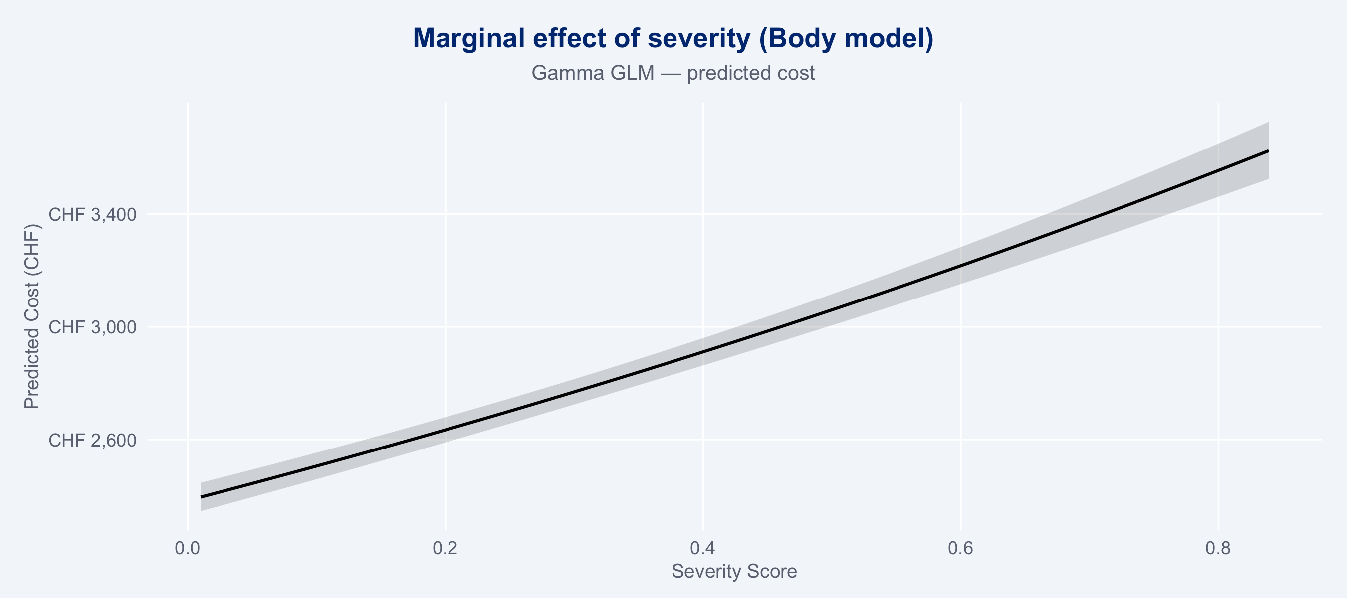
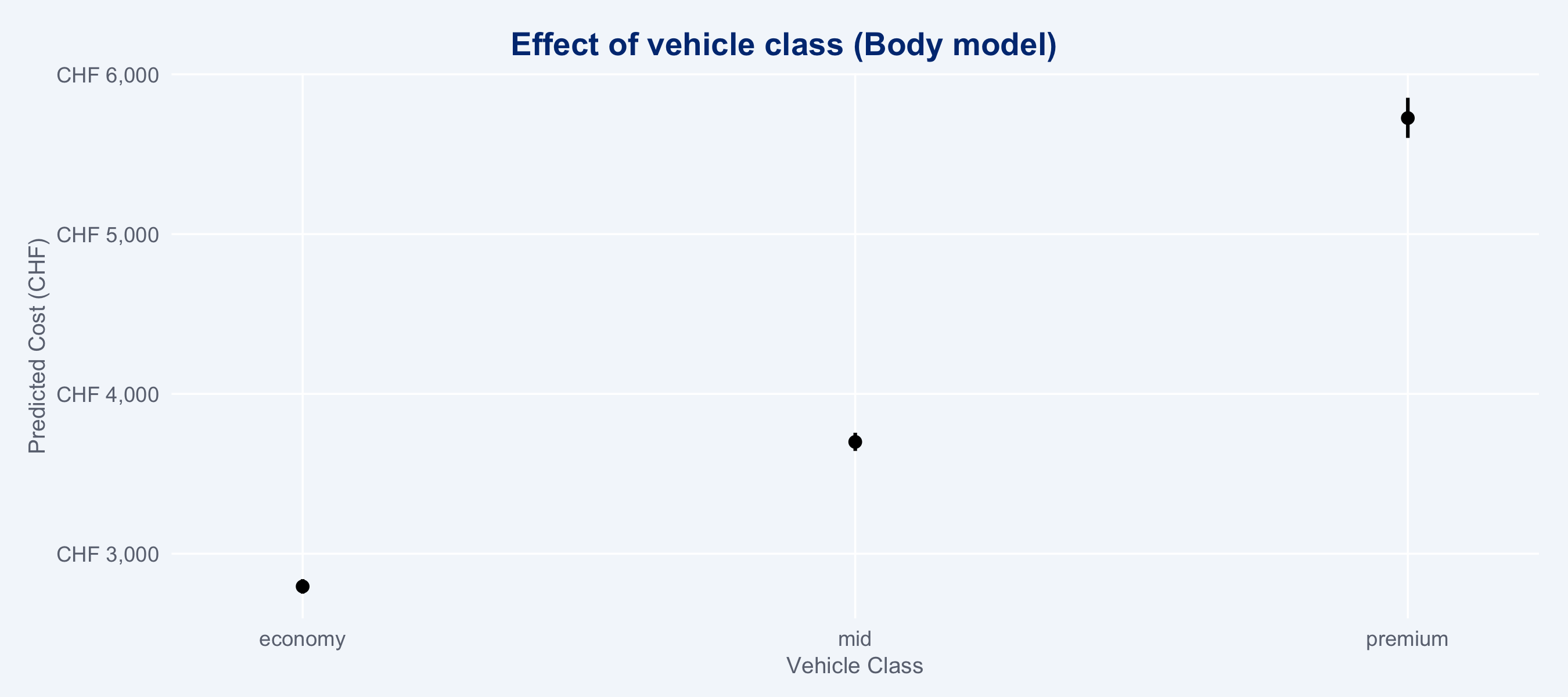
### Marginal Cost Effects (ggeffects)
```{r marginal-effects}
#| fig-height: 4
#| layout-ncol: 2
# Severity effect on cost — body model
gg_sev  <- ggpredict(m_body, terms = "severity_score [all]")
gg_vcls <- ggpredict(m_body, terms = "vehicle_class")

plot(gg_sev) +
  labs(title = "Marginal effect of severity (Body model)",
       subtitle = "Gamma GLM — predicted cost",
       x = "Severity Score", y = "Predicted Cost (CHF)") +
  scale_y_continuous(labels = scales::label_number(prefix = "CHF ", big.mark = ",")) +
  theme_allianz()
plot(gg_vcls) +
  labs(title = "Effect of vehicle class (Body model)",
       x = "Vehicle Class", y = "Predicted Cost (CHF)") +
  scale_y_continuous(labels = scales::label_number(prefix = "CHF ", big.mark = ",")) +
  theme_allianz()
```
### Regression Table (sjPlot)
```{r reg-table}
tbl_body  <- tbl_regression(m_body,  exponentiate = TRUE, label = list(
  vehicle_class  ~ "Vehicle Class",
  vehicle_age    ~ "Vehicle Age",
  severity_score ~ "Severity Score",
  region         ~ "Region"
)) |> bold_p(t = 0.05) |> bold_labels()

tbl_glass <- tbl_regression(models_by_type[["glass"]], exponentiate = TRUE, label = list(
  vehicle_class  ~ "Vehicle Class",
  vehicle_age    ~ "Vehicle Age",
  severity_score ~ "Severity Score",
  region         ~ "Region"
)) |> bold_p(t = 0.05) |> bold_labels()

tbl_merge(
  list(tbl_body, tbl_glass),
  tab_spanner = c("**Body Damage (Gamma GLM)**", "**Glass (Gamma GLM)**")
) |>
  modify_caption("**Regression results** · Exponentiated coefficients (cost ratios)") |>
  as_gt() |>
  tab_style(
    style = cell_fill(color = "#003781"),
    locations = cells_column_labels()
  ) |>
  tab_style(
    style = list(cell_text(color = "white", weight = "bold")),
    locations = cells_column_labels()
  ) |>
  tab_options(table.font.size = px(12))
```
## Observed vs. Expected (O/E) Ratios
```{r oe-ratios}
# Use combined model (all types pooled) for O/E
m_combined <- glm(
  repair_cost ~ claim_type + vehicle_class + vehicle_age + severity_score + region,
  data   = claims_steered,
  family = Gamma(link = "log")
)

oe_df_raw <- observed_vs_expected(m_combined, claims_steered)
oe_df     <- oe_df_raw |>
  left_join(partners |> select(partner_id, name, type, region), by = "partner_id")

# Bootstrap CIs for O/E ratios using mirai (1000 resamples)
cat("Bootstrapping O/E CIs with mirai (500 resamples)...\n")
daemons(4)

boot_results <- mirai_map(
  seq_len(500L),
  function(b, data, partner_ids) {
    idx   <- sample(nrow(data), nrow(data), replace = TRUE)
    d_boot <- data[idx, ]
    m_boot <- glm(
      repair_cost ~ claim_type + vehicle_class + vehicle_age + severity_score + region,
      data = d_boot, family = Gamma(link = "log")
    )
    d_boot$exp_cost <- predict(m_boot, type = "response")
    tapply(seq_len(nrow(d_boot)), d_boot$partner_id, function(i) {
      sum(d_boot$repair_cost[i]) / sum(d_boot$exp_cost[i])
    })
  },
  .args = list(data = claims_steered, partner_ids = oe_df$partner_id)
)

# Extract CI from bootstrap distribution
boot_mat <- do.call(rbind, lapply(boot_results[], function(x) {
  v <- unlist(x)
  v[oe_df$partner_id]
}))

oe_ci <- apply(boot_mat, 2, function(x) quantile(x, c(0.025, 0.975), na.rm = TRUE))
oe_df <- oe_df |>
  mutate(
    oe_boot_lower = oe_ci[1, ],
    oe_boot_upper = oe_ci[2, ]
  )
daemons(0)
```
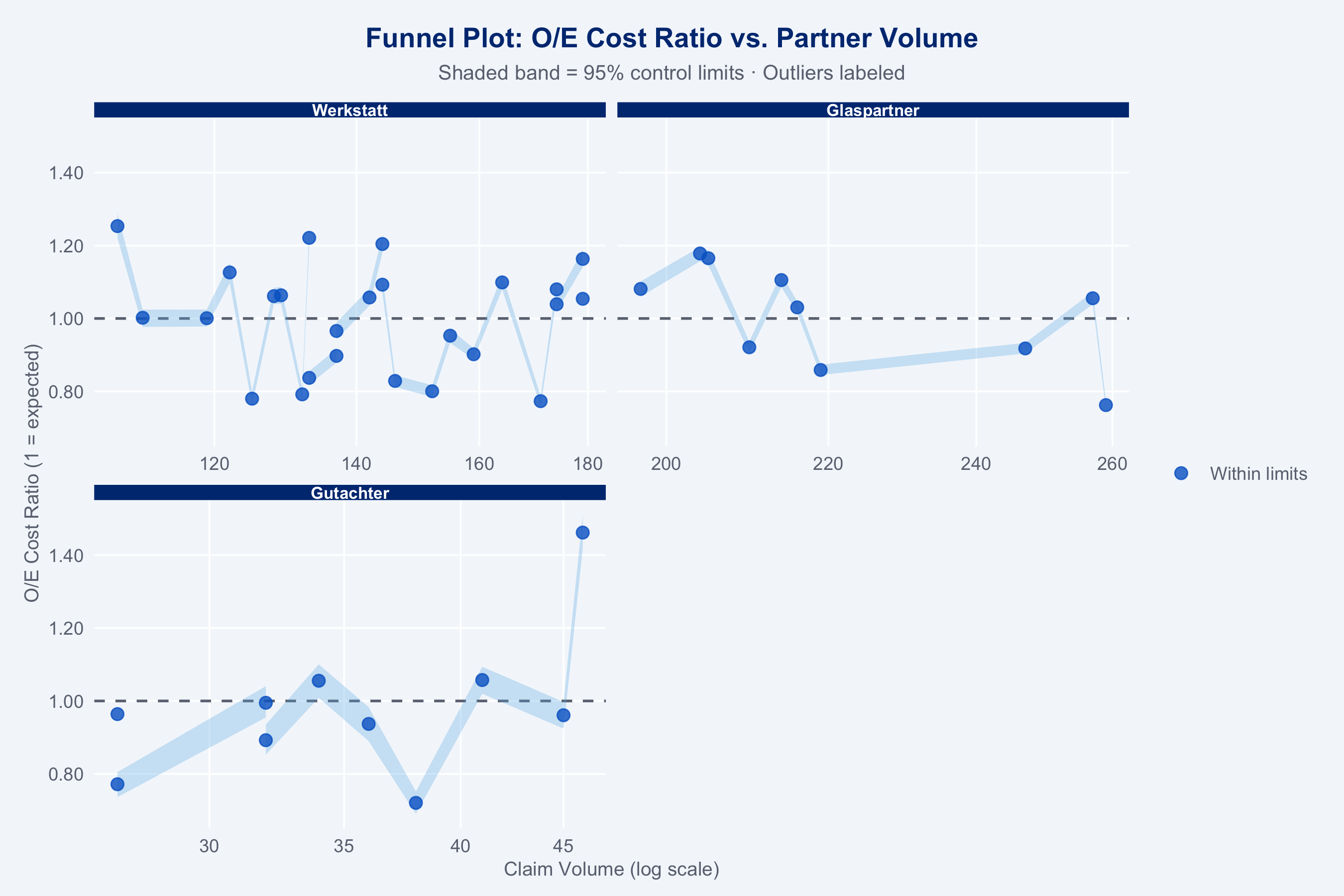
### Funnel Plot
```{r funnel-plot}
#| fig-height: 6
p_funnel <- plot_funnel(
  oe_df |>
    mutate(oe_lower = oe_boot_lower, oe_upper = oe_boot_upper),
  title = "Funnel Plot: O/E Cost Ratio vs. Partner Volume"
)

p_funnel +
  facet_wrap(~type, nrow = 2, scales = "free_x") +
  theme_allianz() +
  theme(strip.text = element_text(size = 8))
```
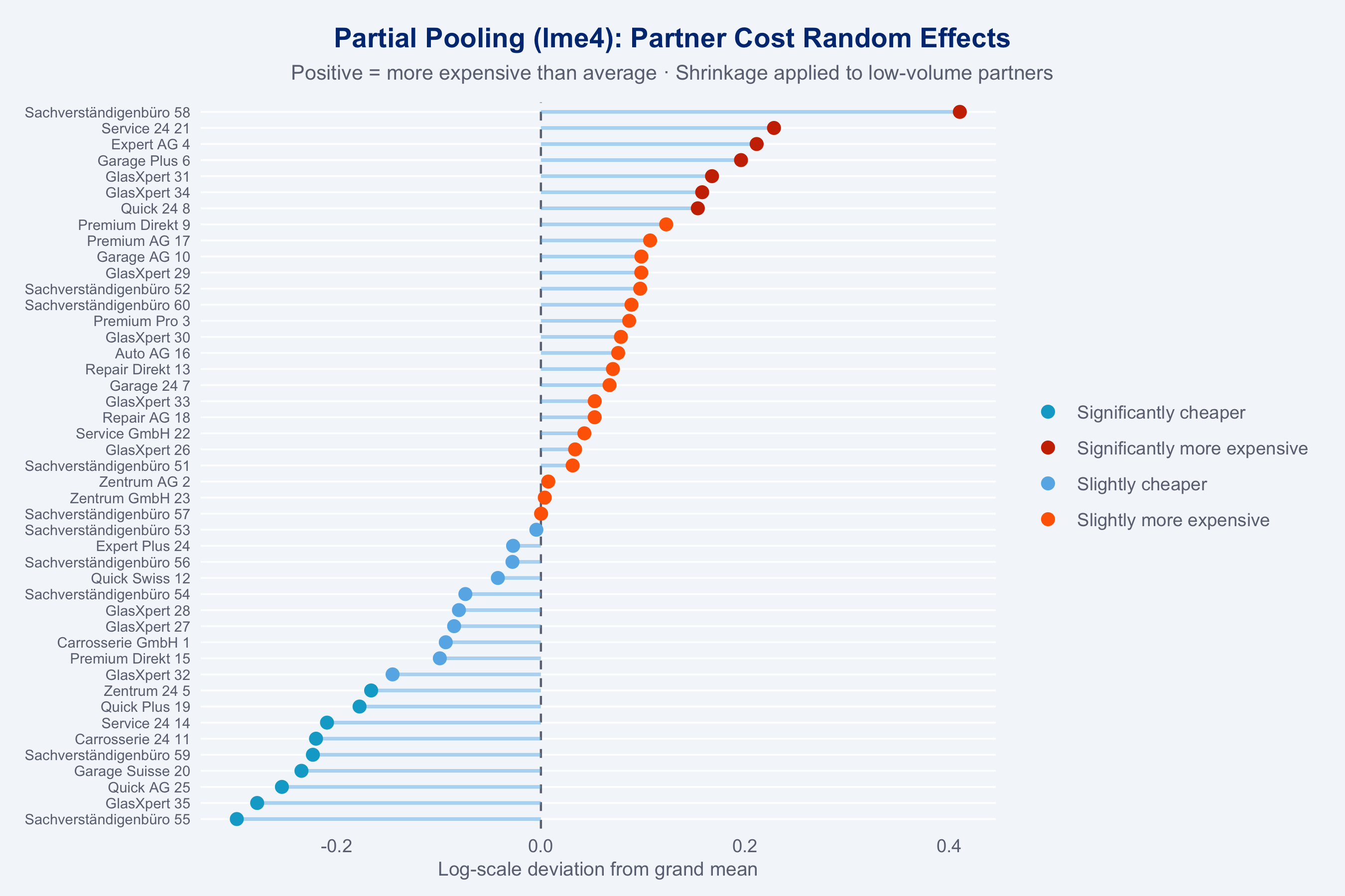
## Partial Pooling (lme4 Shrinkage)
Small-volume partners have noisy raw O/E estimates. Mixed models shrink these toward the
grand mean — a key advantage over naive league tables.
```{r shrinkage}
#| fig-height: 6
ranef_df <- shrinkage_estimate(claims_steered) |>
  left_join(
    claims_steered |>
      count(partner_id) |>
      rename(n_claims = n),
    by = "partner_id"
  ) |>
  left_join(partners |> select(partner_id, name, type), by = "partner_id")

# Plot: random effects (shrunk estimates) sorted
ggplot(ranef_df |> arrange(ranef),
       aes(x = ranef, y = reorder(name, ranef), colour = label)) +
  geom_vline(xintercept = 0, linetype = "dashed", colour = "#6B7280") +
  geom_segment(aes(xend = 0, yend = reorder(name, ranef)),
               colour = "#66B5E8", linewidth = 0.8, alpha = 0.5) +
  geom_point(size = 2.5) +
  scale_colour_manual(
    values = c(
      "Significantly cheaper"         = "#00A9CE",
      "Slightly cheaper"              = "#66B5E8",
      "Slightly more expensive"       = "#FF6600",
      "Significantly more expensive"  = "#CC3300"
    ),
    name = NULL
  ) +
  labs(
    title    = "Partial Pooling (lme4): Partner Cost Random Effects",
    subtitle = "Positive = more expensive than average · Shrinkage applied to low-volume partners",
    x        = "Log-scale deviation from grand mean",
    y        = NULL
  ) +
  theme_allianz(grid = "y") +
  theme(axis.text.y = element_text(size = 7))
```
## Partner League Table
```{r league-table}
kpis        <- compute_kpis(claims, partners)
kpis_cost   <- cost_benchmark(kpis)
speed_df    <- speed_benchmark(claims, partners)
kpis_qual   <- quality_index(kpis_cost)
kpis_full   <- composite_score(kpis_qual, speed_df)

league_tbl <- kpis_full |>
  left_join(oe_df |> select(partner_id, oe_ratio), by = "partner_id") |>
  left_join(ranef_df |> select(partner_id, shrunk_oe), by = "partner_id") |>
  select(name, type, region, n_claims, avg_cost, oe_ratio, shrunk_oe,
         avg_duration, avg_csat, reopen_rate, composite) |>
  arrange(desc(composite))

league_tbl |>
  slice_head(n = 20) |>
  gt() |>
  tab_header(title = "Top 20 Partners — Adjusted League Table",
             subtitle = "Sorted by composite score") |>
  fmt_number(columns = c(avg_cost), decimals = 0, sep_mark = ",") |>
  fmt_number(columns = c(oe_ratio, shrunk_oe), decimals = 3) |>
  fmt_number(columns = c(avg_duration), decimals = 1) |>
  fmt_number(columns = c(avg_csat), decimals = 2) |>
  fmt_percent(columns = reopen_rate, decimals = 1) |>
  fmt_number(columns = composite, decimals = 1) |>
  data_color(
    columns = composite,
    palette = c("#FF6600", "#66B5E8", "#003781")
  ) |>
  tab_style(
    style = cell_fill(color = "#003781"),
    locations = cells_column_labels()
  ) |>
  tab_style(
    style = list(cell_text(color = "white", weight = "bold")),
    locations = cells_column_labels()
  ) |>
  tab_options(table.font.size = px(12))
```
## Model Choice Rationale
**Why Gamma GLM with log link for case-mix adjustment?**
Repair costs are strictly positive and right-skewed — the natural distributional assumption
is Gamma or log-normal, not Gaussian. The Gamma family with a log link ensures positive
predictions at all covariate values (unlike OLS which can predict negative costs) and
handles the multiplicative relationship between covariates and cost correctly. The log link
also makes coefficients interpretable as cost ratios: `exp(β)` gives the multiplicative
change in expected cost per unit change in the predictor.
**Why lme4 partial pooling for shrinkage instead of fixed effects?**
Fixed effects per partner would over-fit to small-volume partners, whose raw O/E ratios are
dominated by sampling noise rather than true performance differences. Random effects (partial
pooling) shrink small-volume partner estimates toward the grand mean proportional to the
reliability of their estimate — mathematically equivalent to Bayesian shrinkage with a normal
prior. This gives fairer rankings: a partner with 10 claims is not penalised for apparent
high cost if it's within the expected noise range.
**Why bootstrap CIs for O/E ratios instead of analytical SEs?**
The O/E ratio is a non-linear function of predicted and observed costs. Analytical standard
errors (delta method) would require assumptions about the joint distribution of predictions —
the bootstrap avoids these assumptions and is valid under mild regularity conditions.
Parallelising 500 resamples via `mirai` makes this computationally tractable.
::: {.callout-note}
**Action items for the Geschäftspartner-Netzwerke team:**
- Partners with O/E > 1.2 **and** n_claims > 50 warrant a formal audit conversation
- Partners with O/E < 0.8 should be examined as potential network expansion candidates
- Re-run this analysis quarterly — seasonal effects (winter bodywork, summer hail) shift rankings
- Extend the adjustment model with `ncd_class`, `coverage_type`, and `fault_indicator`
now that these variables are available in the dataset
:::