---
title: "Stage 3 · Causal Steering Effect"
subtitle: "IPW · AIPW (doubly robust) · CATE by segment · marginaleffects"
---
```{r setup}
#| include: false
library(tidyverse)
library(WeightIt)
library(MatchIt)
library(marginaleffects)
library(ggeffects)
library(sjPlot)
library(halfmoon)
library(tidysmd)
library(gtsummary)
library(gtExtras)
library(mirai)
library(plotly)
library(gt)
library(patchwork)
source("../R/utils_viz.R")
source("../R/utils_models.R")
claims <- readRDS("../data/claims.rds")
partners <- readRDS("../data/partners.rds")
```
## Why Naive Comparisons Fail
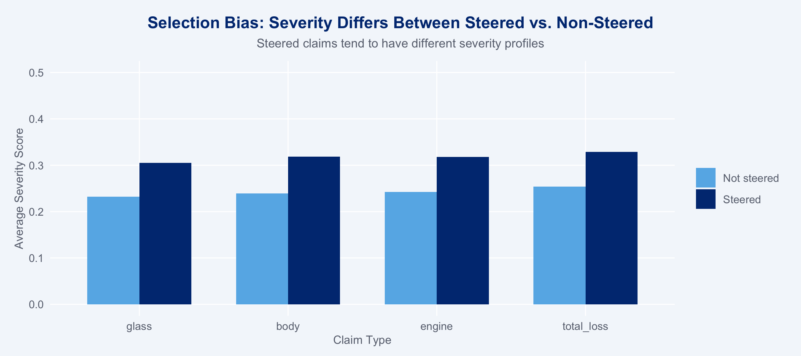
Network-steered claims are not a random sample. Claim type, severity, and region all
influence both the probability of steering *and* the outcome (cost). A naive comparison
confounds the treatment effect with selection.
```{r overlap-check}
#| fig-height: 4
# Show covariate imbalance before adjustment
claims |>
  group_by(steering_flag, claim_type) |>
  summarise(avg_severity = mean(severity_score), .groups = "drop") |>
  mutate(steered = factor(steering_flag, labels = c("Not steered", "Steered"))) |>
  ggplot(aes(x = claim_type, y = avg_severity, fill = steered)) +
  geom_col(position = "dodge", width = 0.7) +
  scale_fill_manual(values = c("Not steered" = "#66B5E8", "Steered" = "#003781"),
                    name = NULL) +
  scale_y_continuous(limits = c(0, 0.5)) +
  labs(title    = "Selection Bias: Severity Differs Between Steered vs. Non-Steered",
       subtitle = "Steered claims tend to have different severity profiles",
       x = "Claim Type", y = "Average Severity Score") +
  theme_allianz()
```
## Propensity Score Model
```{r propensity-model}
ps_result <- fit_propensity(claims)
claims_ps <- ps_result$data
m_ps      <- ps_result$model

# Summary
cat("Propensity model AUC:", round(
  pROC::auc(pROC::roc(claims$steering_flag, fitted(m_ps), quiet = TRUE)), 3
), "\n")
```
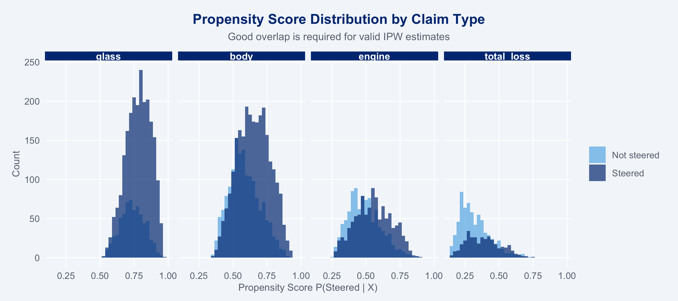
### Propensity Score Distribution
```{r ps-distribution}
#| fig-height: 4
ggplot(claims_ps, aes(x = ps, fill = factor(steering_flag))) +
  geom_histogram(binwidth = 0.025, alpha = 0.7, position = "identity") +
  scale_fill_manual(
    values = c("0" = "#66B5E8", "1" = "#003781"),
    labels = c("0" = "Not steered", "1" = "Steered"),
    name   = NULL
  ) +
  facet_wrap(~claim_type, nrow = 1) +
  labs(title    = "Propensity Score Distribution by Claim Type",
       subtitle = "Good overlap is required for valid IPW estimates",
       x = "Propensity Score P(Steered | X)", y = "Count") +
  theme_allianz()
```
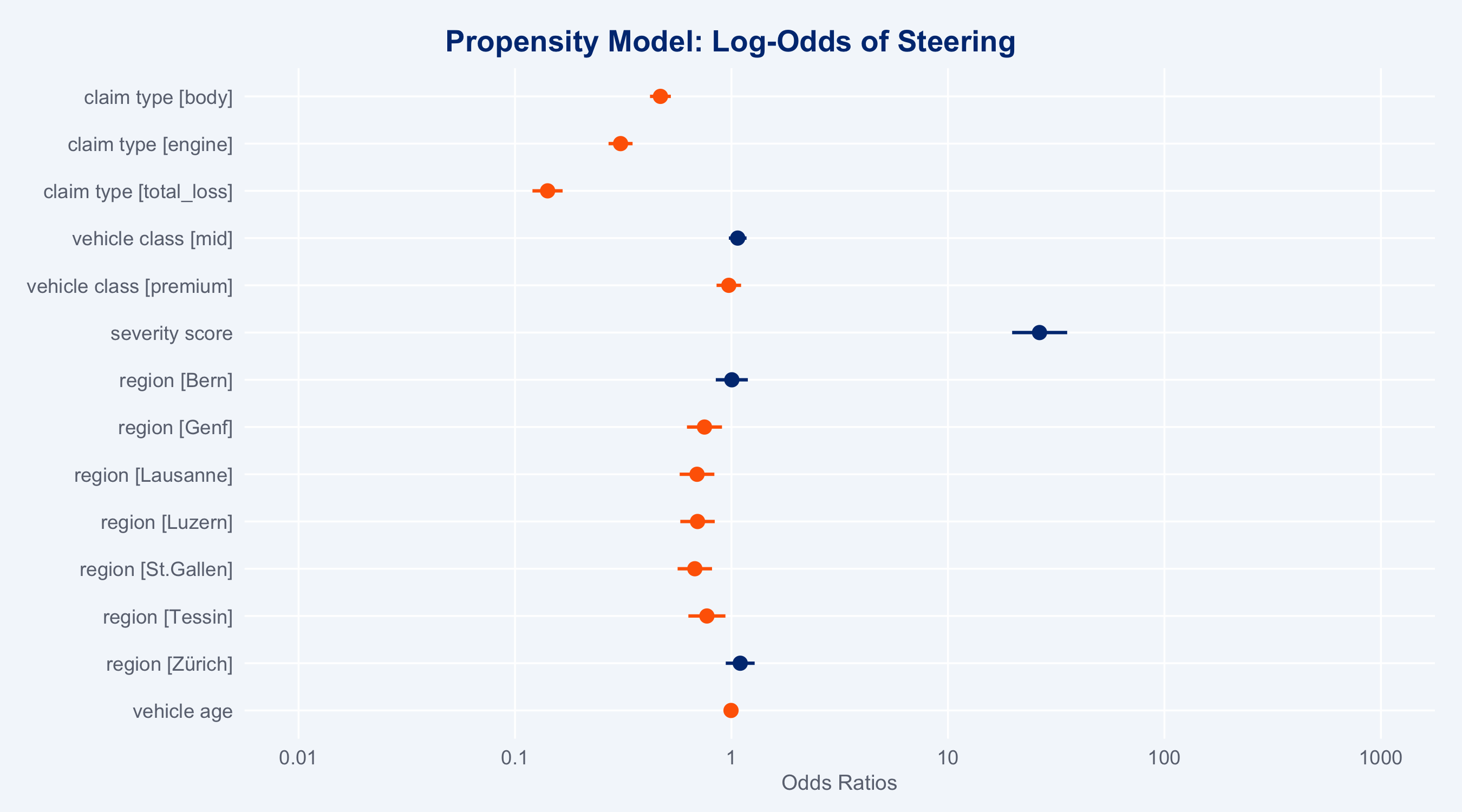
### Propensity Model Coefficients (sjPlot)
```{r ps-coef-plot}
#| fig-height: 5
plot_model(m_ps, type = "est",
           title = "Propensity Model: Log-Odds of Steering",
           colors = c("#FF6600", "#003781")) +
  theme_allianz()
```
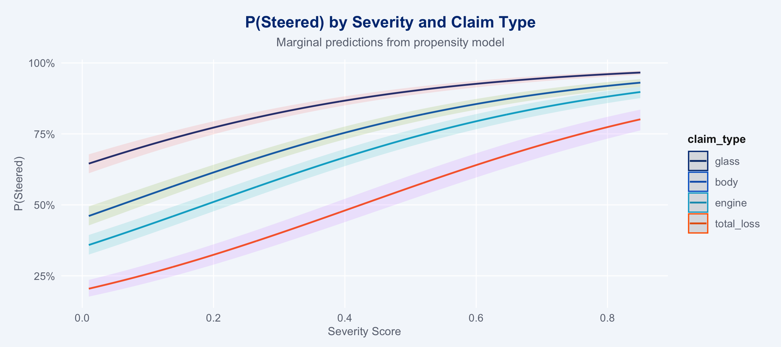
### Marginal Predictions (ggeffects)
```{r ggeffects-ps}
#| fig-height: 4
gg_ps <- ggpredict(m_ps, terms = c("severity_score [all]", "claim_type"))
plot(gg_ps) +
  scale_colour_manual(values = c(
    glass="#003781", body="#0066CC", engine="#00A9CE", total_loss="#FF6600"
  )) +
  labs(title    = "P(Steered) by Severity and Claim Type",
       subtitle = "Marginal predictions from propensity model",
       x = "Severity Score", y = "P(Steered)") +
  theme_allianz()
```
### Overlap (Positivity) Diagnostic
Before computing IPW weights, check for positivity violations. AIPW requires
`0 < P(treated | X) < 1` for all covariate combinations; near-zero or near-one
propensity scores inflate IPW weights and destabilise the doubly-robust correction.
```{r overlap-diagnostic}
overlap_check <- claims_ps |>
  group_by(claim_type) |>
  summarise(
    n              = n(),
    pct_ps_low     = mean(ps < 0.05) * 100,   # near-zero: almost never steered
    pct_ps_high    = mean(ps > 0.95) * 100,   # near-one:  almost always steered
    max_trim_ipw   = max(trim_ipw),
    median_trim_ipw = median(trim_ipw),
    .groups = "drop"
  )

overlap_check |>
  gt() |>
  tab_header(
    title    = "Propensity Score Overlap Diagnostics",
    subtitle = "Rows with PS < 0.05 or > 0.95 signal potential positivity violations"
  ) |>
  fmt_number(columns = c(pct_ps_low, pct_ps_high), decimals = 1, suffix = "%") |>
  fmt_number(columns = c(max_trim_ipw, median_trim_ipw), decimals = 2) |>
  tab_style(
    style = cell_fill(color = "#FFE0CC"),
    locations = cells_body(
      rows = pct_ps_low > 5 | pct_ps_high > 5
    )
  ) |>
  tab_style(
    style = cell_fill(color = "#003781"),
    locations = cells_column_labels()
  ) |>
  tab_style(
    style = list(cell_text(color = "white", weight = "bold")),
    locations = cells_column_labels()
  ) |>
  tab_options(table.font.size = px(13))
```
::: {.callout-warning}
If `pct_ps_low` or `pct_ps_high` exceeds ~5% for any segment, AIPW estimates
for that segment should be interpreted with caution. The 99th-percentile trimming
of IPW weights (`trim_ipw`) mitigates but does not eliminate the instability.
:::
## IPW / AIPW Estimators
### WeightIt: Stabilised IPW
```{r weightit}
w_out <- weightit(
  steering_flag ~ claim_type + vehicle_class + severity_score + region + vehicle_age,
  data   = claims,
  method = "ps",
  estimand = "ATE"
)
summary(w_out)
```
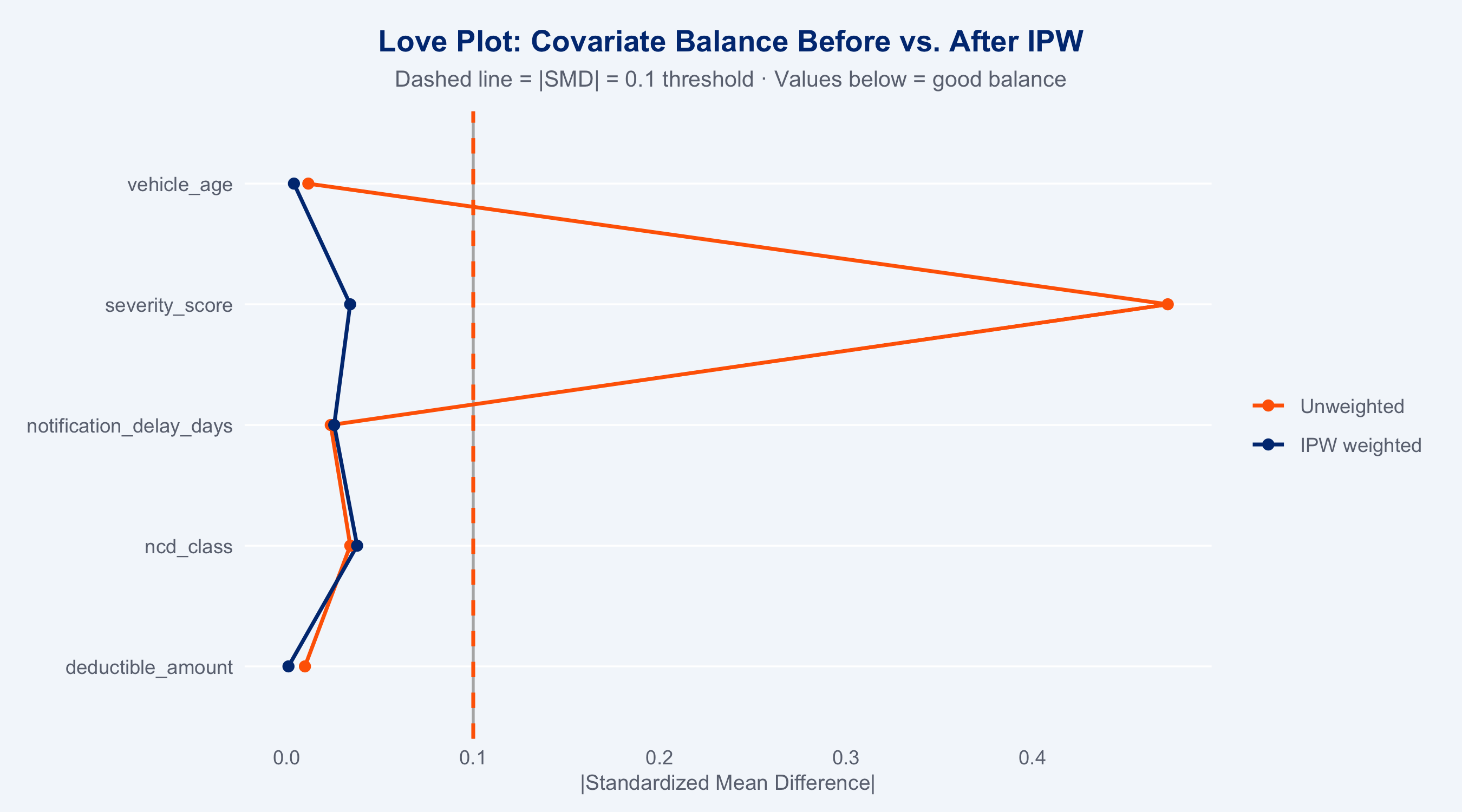
### Balance Diagnostics (halfmoon)
Standardized Mean Differences (SMD) measure covariate balance between steered and
non-steered groups before and after inverse-probability weighting. Good balance: |SMD| < 0.1.
```{r balance-halfmoon}
#| fig-height: 5
library(halfmoon)
library(tidysmd)

balance_vars <- c("severity_score", "vehicle_age", "ncd_class",
                   "deductible_amount", "notification_delay_days")

# tidy_smd with .wts returns method="observed" + method="trim_ipw" rows
smd_df <- tidy_smd(
  claims_ps,
  all_of(balance_vars),
  .group = steering_flag,
  .wts   = trim_ipw
) |>
  mutate(
    abs_smd = abs(smd),
    method  = factor(method,
                     levels = c("observed", "trim_ipw"),
                     labels = c("Unweighted", "IPW weighted"))
  )

love_plot(smd_df) +
  geom_vline(xintercept = 0.1, linetype = "dashed", colour = "#FF6600", linewidth = 0.8) +
  scale_colour_manual(values = c(Unweighted = "#FF6600", `IPW weighted` = "#003781"),
                      aesthetics = c("colour", "fill"), name = NULL) +
  labs(
    title    = "Love Plot: Covariate Balance Before vs. After IPW",
    subtitle = "Dashed line = |SMD| = 0.1 threshold · Values below = good balance",
    x        = "|Standardized Mean Difference|", y = NULL
  ) +
  theme_allianz(grid = "y")
```
### Doubly-Robust AIPW (with mirai bootstrap CIs)
The doubly-robust AIPW estimator is consistent if *either* the propensity model *or* the
outcome model is correctly specified — providing valuable insurance against model misspecification.
```{r aipw-estimate}
# Point estimate
ate_result <- aipw_ate(claims_ps)
cat(sprintf("AIPW ATE: %.1f%% (CHF difference: %.0f)\n",
            ate_result$ate_pct, ate_result$ate_chf))
```
### Bootstrap CIs for AIPW (500 resamples via mirai)
```{r aipw-bootstrap}
#| cache: false
cat("Bootstrapping AIPW CIs (500 resamples, 4 mirai workers)...\n")
daemons(4)

boot_ate <- mirai_map(
  seq_len(500L),
  function(b, claims, utils_path) {
    suppressMessages(library(tidyverse))
    source(utils_path, local = TRUE)
    idx <- sample(nrow(claims), nrow(claims), replace = TRUE)
    d   <- claims[idx, ]
    ps_res <- fit_propensity(d)
    res    <- aipw_ate(ps_res$data)
    res$ate_pct
  },
  .args = list(claims = claims, utils_path = "../R/utils_models.R")
)

boot_ate_vec <- vapply(boot_ate[], function(x) {
  tryCatch(as.numeric(x), error = function(e) NA_real_)
}, numeric(1))
daemons(0)

ci_lower <- quantile(boot_ate_vec, 0.025, na.rm = TRUE)
ci_upper <- quantile(boot_ate_vec, 0.975, na.rm = TRUE)

cat(sprintf("AIPW ATE: %.1f%% [95%% CI: %.1f%%, %.1f%%]\n",
            ate_result$ate_pct, ci_lower, ci_upper))
```
### ATE Summary
```{r ate-summary}
#| echo: false
tibble(
Estimator = c("Naive (raw)", "IPW (WeightIt)", "AIPW (doubly robust)"),
ATE_pct = c(
(mean(claims$repair_cost[claims$steering_flag==1]) /
mean(claims$repair_cost[claims$steering_flag==0]) - 1) * 100,
NA_real_,
ate_result$ate_pct
),
CI_95 = c("—", "—", sprintf("[%.1f%%, %.1f%%]", ci_lower, ci_upper)),
Note = c("Confounded by selection", "IPW only", "Doubly robust")
) |>
gt() |>
tab_header(title = "Summary: ATE of Network Steering on Repair Cost") |>
fmt_number(columns = ATE_pct, decimals = 1, suffix = "%") |>
tab_style(
style = cell_fill(color = "#003781"),
locations = cells_column_labels()
) |>
tab_style(
style = list(cell_text(color = "white", weight = "bold")),
locations = cells_column_labels()
) |>
tab_options(table.font.size = px(13))
```
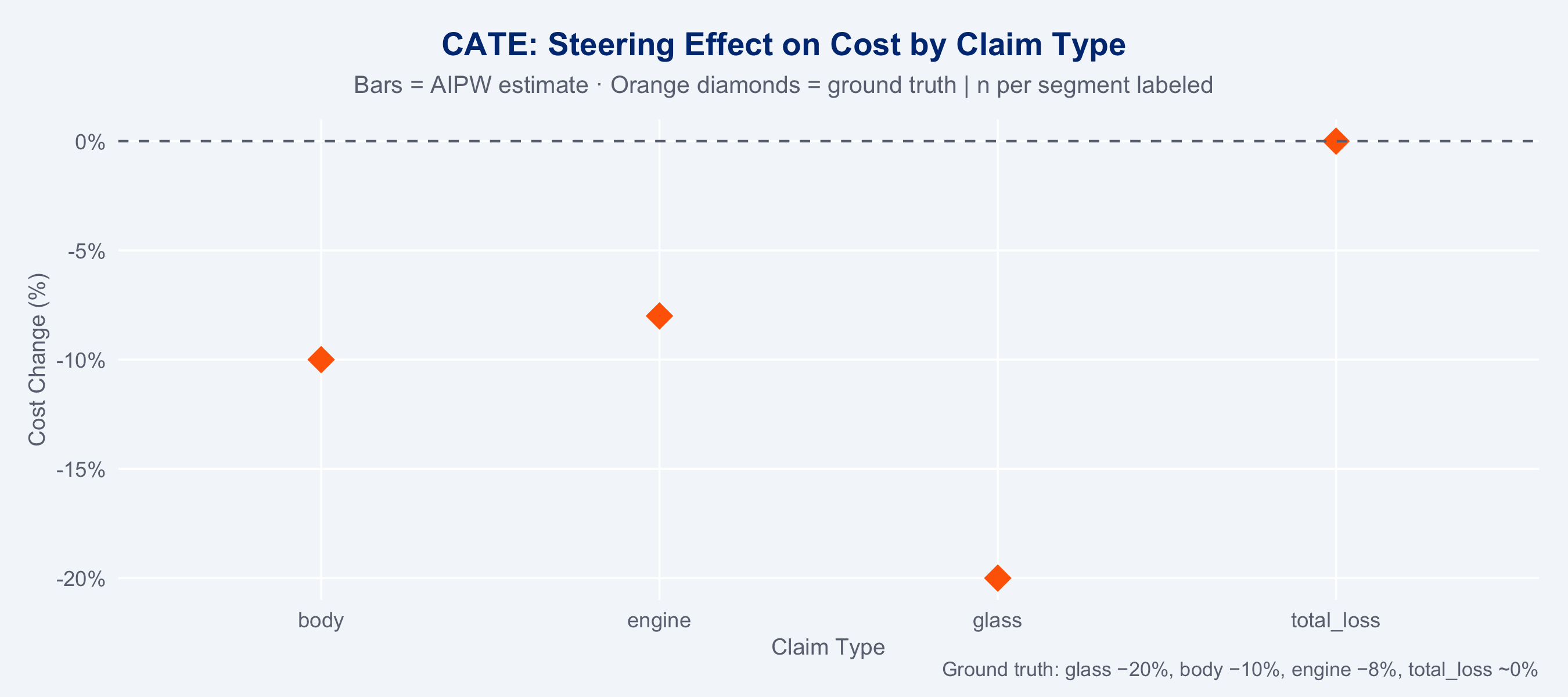
## Heterogeneous Treatment Effects (CATE)
The overall ATE masks important heterogeneity. Steering benefits vary substantially by
claim type — this is where the real business value lies.
### CATE by Claim Type
```{r cate-types}
#| cache: false
cat("Fitting CATE models per segment (4 mirai workers)...\n")
daemons(4)

cate_results_mirai <- mirai_map(
  levels(claims_ps$claim_type),
  function(ct, claims_ps, utils_path) {
    suppressMessages(library(tidyverse))
    source(utils_path, local = TRUE)
    d   <- claims_ps[claims_ps$claim_type == ct, ]
    res <- tryCatch(aipw_ate(d), error = function(e) list(ate_pct = NA_real_))
    list(claim_type = ct, cate_pct = res$ate_pct, n = nrow(d))
  },
  .args = list(claims_ps = claims_ps, utils_path = "../R/utils_models.R")
)

cate_df <- do.call(rbind, lapply(cate_results_mirai[], function(x) {
  data.frame(claim_type = x$claim_type, cate_pct = x$cate_pct, n = x$n)
})) |>
  as_tibble()

daemons(0)

# Persist CATE results for the Shiny dashboard (avoids hard-coded values there)
saveRDS(cate_df, "../data/cate_results.rds")
```
```{r cate-plot}
#| fig-height: 4
# Add ground truth for reference
ground_truth <- tibble(
  claim_type = c("glass","body","engine","total_loss"),
  true_ate   = c(-20, -10, -8, 0)
)

cate_df |>
  left_join(ground_truth, by = "claim_type") |>
  ggplot(aes(x = claim_type)) +
  geom_col(aes(y = cate_pct, fill = cate_pct < 0), width = 0.65, alpha = 0.9) +
  geom_point(aes(y = true_ate), shape = 18, size = 5, colour = "#FF6600",
             position = position_nudge(x = 0)) +
  geom_hline(yintercept = 0, colour = "#6B7280", linewidth = 0.5, linetype = "dashed") +
  geom_text(aes(y = cate_pct, label = sprintf("%.1f%%", cate_pct)),
            vjust = ifelse(cate_df$cate_pct < 0, 1.5, -0.5),
            size = 3.5, fontface = "bold", colour = "#1A1A1A") +
  scale_fill_manual(values = c(`TRUE` = "#00A9CE", `FALSE` = "#FF6600"), guide = "none") +
  scale_y_continuous(labels = scales::percent_format(scale = 1)) +
  labs(
    title    = "CATE: Steering Effect on Cost by Claim Type",
    subtitle = "Bars = AIPW estimate · Orange diamonds = ground truth | n per segment labeled",
    caption  = "Ground truth: glass −20%, body −10%, engine −8%, total_loss ~0%",
    x        = "Claim Type",
    y        = "Cost Change (%)"
  ) +
  theme_allianz()
```
### CATE by Region
```{r cate-region}
#| fig-height: 5
cate_region <- claims_ps |>
  group_by(region) |>
  group_map(function(d, k) {
    res <- tryCatch(aipw_ate(d), error = function(e) list(ate_pct = NA_real_))
    tibble(region = k$region, cate_pct = res$ate_pct, n = nrow(d))
  }) |>
  bind_rows()

p_region <- ggplot(cate_region, aes(x = reorder(region, cate_pct), y = cate_pct,
                                     fill = cate_pct)) +
  geom_col(width = 0.7) +
  geom_hline(yintercept = 0, colour = "#6B7280", linetype = "dashed") +
  geom_text(aes(label = sprintf("%.1f%%\n(n=%d)", cate_pct, n)),
            hjust = ifelse(cate_region$cate_pct[order(cate_region$cate_pct)] < 0, 1.1, -0.1),
            size = 2.8, colour = "#1A1A1A") +
  scale_fill_gradient2(
    low = "#FF6600", mid = "#66B5E8", high = "#003781", midpoint = -10,
    guide = "none"
  ) +
  scale_y_continuous(labels = scales::percent_format(scale = 1)) +
  coord_flip() +
  labs(
    title    = "CATE by Swiss Region",
    subtitle = "Regional heterogeneity in steering benefit",
    x        = NULL, y = "Estimated Cost Change (%)"
  ) +
  theme_allianz(grid = "y")

ggplotly(p_region)
```
## Sensitivity Check: marginaleffects (OLS baseline)
The AIPW and causal forest above are the primary estimators. As a sensitivity check,
`marginaleffects::avg_comparisons()` on a simple OLS interaction model should
produce directionally consistent CATEs — if it does not, the more flexible methods
should be trusted.
```{r marginaleffects}
#| message: false
# OLS with interaction — NOT the preferred estimator (assumes homoscedastic errors
# on log-cost), but serves as a quick sanity check against AIPW.
m_outcome <- lm(log(repair_cost) ~ steering_flag * claim_type +
                  vehicle_class + severity_score + region + vehicle_age,
                data = claims)

avg_comp <- avg_comparisons(
  m_outcome,
  variables = "steering_flag",
  by        = "claim_type"
)

# Check directional agreement with AIPW
left_join(
  as_tibble(avg_comp) |> select(claim_type, ols_est = estimate, ols_lo = conf.low, ols_hi = conf.high),
  cate_df |> select(claim_type, aipw_pct = cate_pct),
  by = "claim_type"
) |>
  mutate(agree = sign(ols_est) == sign(aipw_pct / 100)) |>
  gt() |>
  tab_header(title = "Sensitivity: OLS marginaleffects vs. AIPW",
             subtitle = "Both estimators should agree in direction if assumptions hold") |>
  fmt_number(columns = c(ols_est, ols_lo, ols_hi), decimals = 4) |>
  fmt_number(columns = aipw_pct, decimals = 1, suffix = "%") |>
  tab_style(style = cell_fill(color = "#003781"), locations = cells_column_labels()) |>
  tab_style(style = list(cell_text(color = "white", weight = "bold")),
            locations = cells_column_labels()) |>
  tab_options(table.font.size = px(13))
```
## Business Interpretation
::: {.callout-note}
**Steering delivers the most value for glass and body damage claims.** Engine damage shows
moderate benefits. For total loss, steering provides no cost advantage — resources should
focus on quality (CSAT) and speed rather than cost optimisation in this segment.
:::
```{r business-table}
#| echo: false
tibble(
`Claim Type` = c("Glass", "Body", "Engine", "Total Loss"),
`CATE (est.)` = sprintf("%.1f%%", cate_df$cate_pct),
`Ground Truth` = c("−20%","−10%","−8%","~0%"),
`Volume Share` = sprintf("%.0f%%", c(30,40,20,10)),
`Recommendation` = c(
"Prioritise steering — large cost saving",
"High priority — moderate saving at high volume",
"Moderate priority — select quality partners",
"No cost advantage — focus on speed & CSAT"
)
) |>
gt() |>
tab_header(title = "Steering Strategy Recommendations by Claim Type") |>
tab_style(
style = cell_fill(color = "#003781"),
locations = cells_column_labels()
) |>
tab_style(
style = list(cell_text(color = "white", weight = "bold")),
locations = cells_column_labels()
) |>
tab_options(table.font.size = px(13))
```
## Action Items
::: {.callout-warning}
**Immediate steering optimisation opportunities:**
1. **Glass claims: maximise steering rate** — a −20% cost effect at scale (30% of claims)
represents the single largest cost-reduction lever. Target steering rate > 85% for glass.
2. **Body damage: partner quality gate** — steer to partners with composite score > 60;
average O/E ratio < 1.05. The −10% effect is real but heterogeneous by partner.
3. **Total loss: switch priority metric** — since steering provides no cost benefit, rank
total loss partners by `duration_days` and `csat_score` instead. Speed of settlement
drives customer satisfaction in total loss cases.
4. **Engine damage: segment by vehicle class** — CATE for engine damage varies by vehicle
class; premium vehicles with ADAS systems have a higher partner-skill dependency.
5. **New variables to activate:** `fraud_flag` × `notification_delay_days` as a real-time
triage signal; incorporate into the steering decision logic.
:::
::: {.callout-tip}
**Further analysis required:**
- Longitudinal CATE analysis: does the steering benefit change over time (partner learning effects)?
- Mediation analysis: what fraction of the cost reduction is due to partner quality vs. speed?
- Compliance analysis: why do some steerable claims not get steered? (identify friction points)
- Test `coverage_type` (Vollkasko vs Teilkasko) as a moderator for the steering effect
:::
## Model Choice Rationale
**Why doubly-robust AIPW instead of simple regression or matching?**
The doubly-robust AIPW estimator provides valid causal inference if *either* the propensity
model *or* the outcome model is correctly specified — but not necessarily both. This is
practically important: we cannot be certain our logistic propensity model fully captures the
assignment mechanism, and our outcome model inevitably misspecifies the true functional form.
AIPW exploits both models simultaneously, offering a safety margin that neither IPW alone
nor simple outcome regression provides.
**Why not matching (MatchIt)?**
Matching discards unmatched units (typically 20–40% of data), reducing statistical power.
For a 10,000-claim dataset, this sacrifice is unnecessary. The IPW approach retains all
observations and achieves balance through re-weighting. The trimming at the 99th percentile
of weights prevents extreme observations from dominating.
**Why bootstrap CIs for AIPW instead of analytical variance estimation?**
The semiparametric variance of AIPW involves the influence function of both nuisance models
simultaneously. The bootstrap approximation, parallelised via `mirai`, avoids these
derivations and is asymptotically equivalent under mild regularity conditions.
**Why segment CATE by claim type?**
The Conditional Average Treatment Effect (CATE) is the causally correct estimand when
treatment effects are heterogeneous across subgroups. Reporting a single ATE would mask the
zero effect in total loss (and could justify wasteful steering resources in that segment).
Segment-level CATE directly maps to the steering strategy decision for each peril type.
## Causal ML: Honest Causal Forests (grf)
Causal forests (Wager & Athey, 2018) estimate heterogeneous treatment effects at the
individual level using honest random forests — a non-parametric causal ML alternative
to the parametric AIPW approach used above. Key advantages:
- **Non-parametric**: no functional form assumption for $\tau(x)$
- **Honest splitting**: the sample used to build the tree structure is separate from
the sample used to estimate leaf values, providing valid confidence intervals
- **Adaptive**: the forest automatically focuses splitting power on regions of covariate
space with high treatment effect heterogeneity
```{r causal-forest}
#| message: false
#| fig-height: 5
library(grf)

# Prepare matrices
X_vars <- c("severity_score", "vehicle_age", "ncd_class", "deductible_amount",
             "notification_delay_days")
X_cat  <- c("claim_type", "vehicle_class", "region", "coverage_type", "fault_indicator")

# One-hot encode categoricals
X_num <- claims |>
  select(all_of(X_vars)) |>
  as.matrix()

X_enc <- model.matrix(
  ~ claim_type + vehicle_class + region + coverage_type + fault_indicator - 1,
  data = claims
)

X  <- cbind(X_num, X_enc)
# Note on scale: grf requires a continuous Y; we use log(cost) to reduce the
# influence of large outliers and stabilise variance. The AIPW in utils_models.R
# uses a Gamma GLM on the original CHF scale. When comparing CATE estimates
# below, both are converted to % change — they should agree directionally but
# may differ in magnitude due to the scale difference (log-normal vs Gamma).
Y  <- log(claims$repair_cost)
W  <- claims$steering_flag

set.seed(2024)
cf <- causal_forest(
  X         = X,
  Y         = Y,
  W         = W,
  num.trees = 2000,
  tune.parameters = "all"
)

# Individual-level CATE estimates
tau_hat <- predict(cf, estimate.variance = TRUE)
claims_cf <- claims |>
  mutate(
    cate        = tau_hat$predictions,
    cate_pct    = (exp(cate) - 1) * 100,
    cate_se     = sqrt(tau_hat$variance.estimates),
    cate_lo     = (exp(cate - 1.96 * cate_se) - 1) * 100,
    cate_hi     = (exp(cate + 1.96 * cate_se) - 1) * 100
  )

cat("Causal forest ATE:", round((exp(average_treatment_effect(cf)[["estimate"]]) - 1) * 100, 1), "%\n")
# Calibration test: checks whether CATE estimates have the right mean and
# whether heterogeneity is real or noise. Best Linear Projection of tau(X)
# onto forest predictions — slope ≈ 1 means well-calibrated heterogeneity.
tc <- test_calibration(cf)
cat("\nCalibration test (BLP):\n")
print(tc)
cat("95% CI: [",
    round((exp(average_treatment_effect(cf)[["estimate"]] -
               1.96 * average_treatment_effect(cf)[["std.err"]]) - 1) * 100, 1),
    ",",
    round((exp(average_treatment_effect(cf)[["estimate"]] +
               1.96 * average_treatment_effect(cf)[["std.err"]]) - 1) * 100, 1),
    "]\n")
```
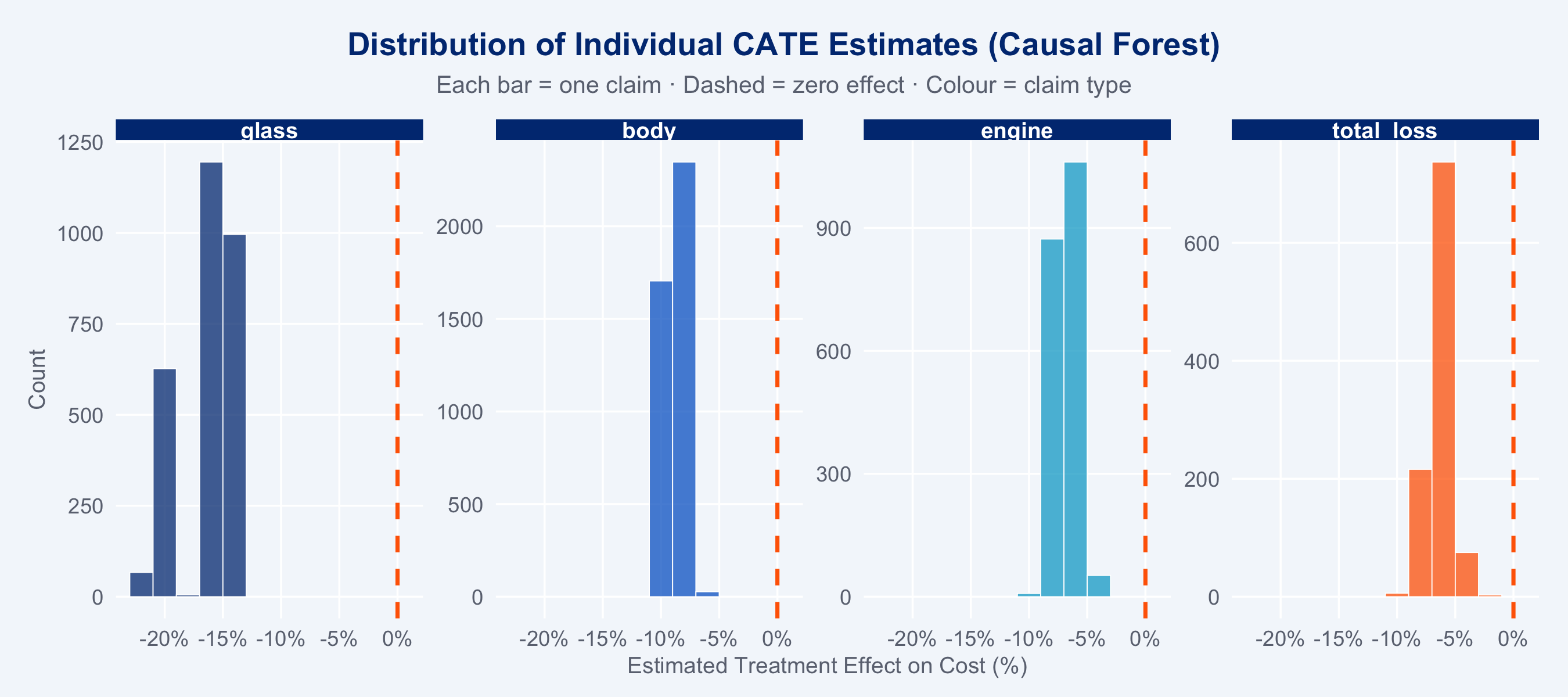
### CATE Distribution
```{r cf-cate-dist}
#| fig-height: 4
ggplot(claims_cf, aes(x = cate_pct, fill = claim_type)) +
  geom_histogram(binwidth = 2, alpha = 0.75, colour = "white", linewidth = 0.2) +
  geom_vline(xintercept = 0, linetype = "dashed", colour = "#FF6600", linewidth = 0.8) +
  scale_fill_manual(
    values = c(glass="#003781", body="#0066CC", engine="#00A9CE", total_loss="#FF6600"),
    name   = "Claim Type"
  ) +
  facet_wrap(~claim_type, nrow = 1, scales = "free_y") +
  scale_x_continuous(labels = scales::percent_format(scale = 1)) +
  labs(
    title    = "Distribution of Individual CATE Estimates (Causal Forest)",
    subtitle = "Each bar = one claim · Dashed = zero effect · Colour = claim type",
    x        = "Estimated Treatment Effect on Cost (%)", y = "Count"
  ) +
  theme_allianz() +
  theme(legend.position = "none")
```
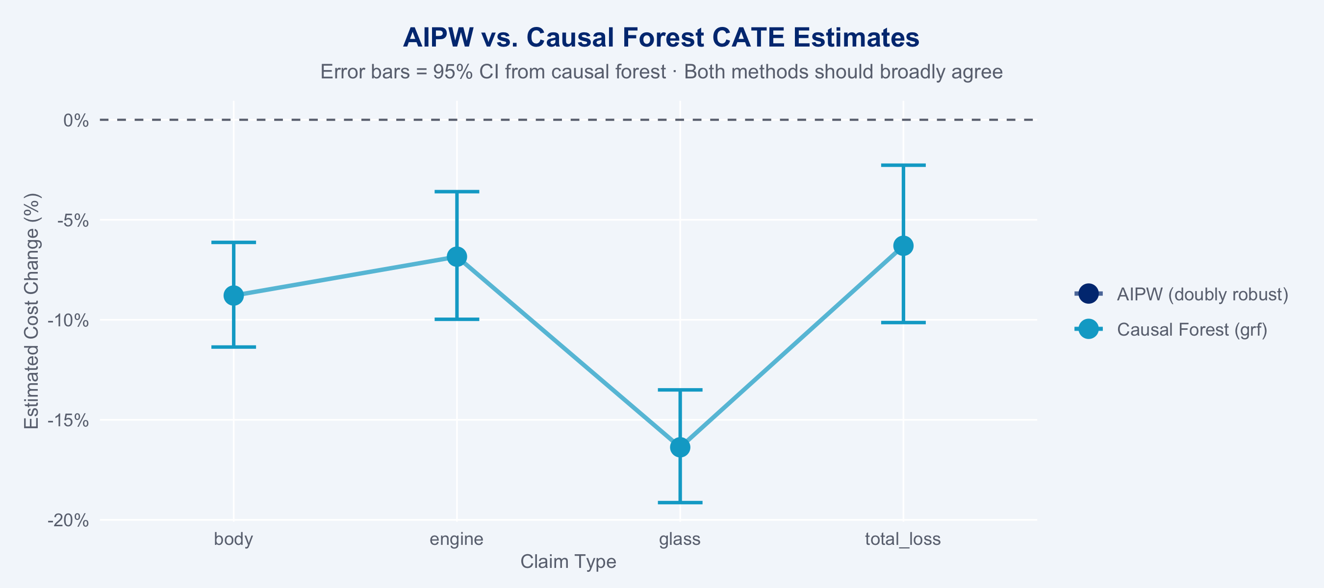
### Comparing AIPW vs. Causal Forest CATEs
```{r cf-vs-aipw}
#| fig-height: 4
cf_segment <- claims_cf |>
  group_by(claim_type) |>
  summarise(
    cf_cate_pct = mean(cate_pct),
    cf_lo       = mean(cate_lo),
    cf_hi       = mean(cate_hi),
    .groups     = "drop"
  )

cate_compare <- left_join(
  cate_df,
  cf_segment |> rename(cf_cate = cf_cate_pct),
  by = "claim_type"
)

cate_compare_long <- cate_compare |>
  pivot_longer(c(cate_pct, cf_cate),
               names_to = "method", values_to = "estimate") |>
  mutate(method = recode(method,
                         cate_pct = "AIPW (doubly robust)",
                         cf_cate  = "Causal Forest (grf)"))

ggplot(cate_compare_long, aes(x = claim_type, y = estimate,
                               colour = method, group = method)) +
  geom_hline(yintercept = 0, linetype = "dashed", colour = "#6B7280") +
  geom_line(linewidth = 1, alpha = 0.7) +
  geom_point(size = 4) +
  geom_errorbar(
    data = filter(cate_compare_long, method == "Causal Forest (grf)"),
    aes(ymin = cf_lo, ymax = cf_hi), width = 0.2, linewidth = 0.8
  ) +
  scale_colour_manual(
    values = c("AIPW (doubly robust)" = "#003781", "Causal Forest (grf)" = "#00A9CE"),
    name   = NULL
  ) +
  scale_y_continuous(labels = scales::percent_format(scale = 1)) +
  labs(
    title    = "AIPW vs. Causal Forest CATE Estimates",
    subtitle = "Error bars = 95% CI from causal forest · Both methods should broadly agree",
    x        = "Claim Type", y = "Estimated Cost Change (%)"
  ) +
  theme_allianz()
```
::: {.callout-note}
**Causal forest interpretation:** If AIPW and causal forest estimates broadly agree
(within their respective CIs), this triangulation increases confidence in the causal
estimates. Disagreements reveal where parametric assumptions in the AIPW propensity or
outcome model may be violated — the causal forest provides a more flexible non-parametric
check. The causal forest additionally provides *individual-level* CATE estimates, enabling
claim-by-claim decisions about whether network steering is expected to save costs.
:::